Example: Employee Selection
This is an example of a simple didactic DEX model aimed at the assessment of applicants for a Project Manager position in a small company. In contrast with the Car Evaluation example, this particular model contains two continuous attributes and two discretization functions, and can be thus fully utilized only in DEXi Suite. All figures and charts on this page have been generated using DEXiWin.
Tree of Attributes
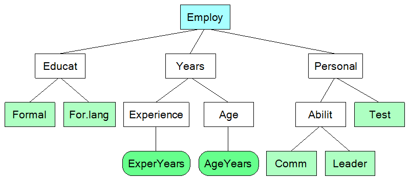
The Employee Selection model has the following tree structure of attributes:
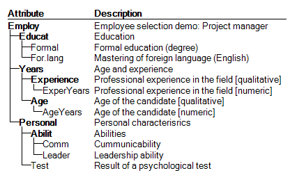
The same structure, displayed with descriptions of attributes:
Notice that attributes ExperYears and AgeYears are continuous. In the model, they are discretized and mapped to their respective parents, Experience and Age.
Scales
The scales of attributes are defined as follows:
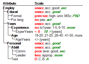
Apart from the two continous scales, ExperYears and AgeYears, all the remaining scales are qualitative. Among these, Age is unordered, and all the others are preferentially ordered in the ascending order.
Most of the qualitative values are represented by words: ‘unacc’, ‘high’, etc. Even though some values, for instance ‘1–5’ and ‘21–25’, are formulated as numeric intervals, they still represent single qualitative symbols.
The symbol ‘<>’ denotes an unordered continuous scale of AgeYears. The continuous scale of ExperYears, denoted ‘<0; 10>’, is preferentially ordered and has two bounds: 0 and 10. All values below and including 0 are considered preferentially ‘bad’, and all values above and including 10 are considered ‘good’.
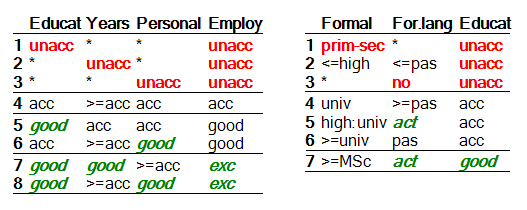
Aggregation Functions
The Employee Selection model contains seven qualitative attributes: Employ, Educat, Years, Personal, Abilit, Experience, and Age. The former five of them are associated with aggregation functions. For brevity, only two of those are shown below in the form of complex decision rules.
Discretization Functions
Discretization functions map numeric values of continuous input attributes to the qualitative values of the corresponding parent attributes. The two discretization function in the Employee Selection model are associated with Experience and Age, and are defined as follows:
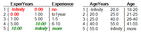
Notice the symbols ‘[’, ‘]’, ‘(’ and ‘)’, associated with intervals:
‘[’ and ‘]’ denote the closed interval, so that the corresponding value belongs to the interval
‘(’ and ‘)’ denote the open interval, so that the associated value does not belong to that interval, but to the neighboring one
Description of Employees
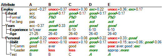
Alternatives - employee candidates - are defined by values of input (basic) attributes as follows:
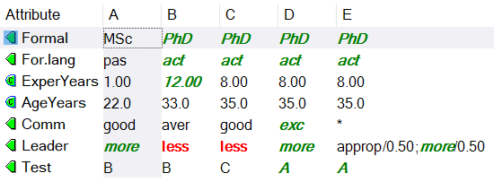
There are five candidates, named A, B, C, D, and E. The former four are represented by single values, assigned to the five qualitative and two continuous input attributes.
The candidate E is an exception, aimed at illustrating the use of other types of DEX values. The asterisk ‘*’ denotes the whole set of values of the corresponding attribute Comm, indicating that nothing is known about E’s communicative abilities. The value of Leader is also somewhat uncertain, described by the value distribution ‘approp/0.50; more/0.50’. This distribution is interpreted later in the evaluation either as a probability or fuzzy distribution, but the basic interpretation is that E’s leadership abilities are assessed as ‘appropriate’ or ‘more’ (with equal strength), but not ‘less’.
Evaluation of Employees
The above five employee candidates are evaluated, using the probabilistic value interpretation and evaluation method, as follows:
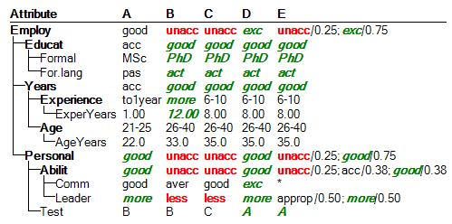
The final evaluations are: candidate A is ‘good’, candidates B and C are ‘unacc’, candidate D is ‘exc’, and the evaluation of candidate E is a probability distribution of ‘unacc’ (with probability 0.25) and ‘exc’ (0.75).
In order to explain why the evaluations are such, one can look at the respective columns and inspect lower-level values that affected the evaluation.
Analysis of Employees
Selective explanation
Selective explanation highlights particular advantages and disadvantages of an alternative. The method finds and displays only those connected sub-trees of attributes for which the alternative has been evaluated as particularly good or bad.
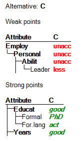
This example shows that candidate C has both weak and strong points. Her particular weakness is Leader, which is ‘less’ and largely affects the ‘unacc’ evaluation of Employ. On the other hand, the candidate is very strong regarding her Educat (both Formal and For. lang) and Years (age and experience).
Plus-minus analysis
This is an example of “Plus-minus analysis” of candidate A:
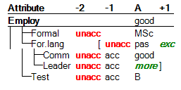
Overall, candidate A has been evaluated as ‘good’, as shown in the first row. Column +1 shows that evaluation can be improved by one step (i.e., to ‘exc’) only by changing the value of For. lang by one step (from ‘pas’ to ‘act’); in this case, the overall evaluation would become ‘exc’. In a similar way, the columns -1 and -2 show the overall evaluation results when the corresponding attributes (only one at a time) change by one or two steps, respectively.
The brackets ‘[’ and ‘]’ indicate that the values of the corresponding attributes (For. lang and Leader) cannot be changed by the requested number of steps.
Target Analysis
Target analysis tries to find the smallest changes of input values that improve or degrade the value of some selected aggregate attribute. In contrast with Plus-Minus analysis, possible changes of more than one attribute at a time are observed. The following example shows the results of Target Analysis for candidate C:
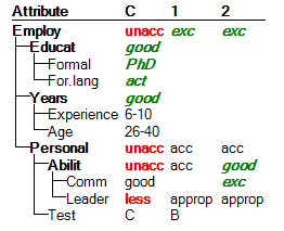
There are two possible ways of improving his evaluation:
improving Leader from ‘less’ to ‘approp’ and Test from C to B
improving Comm from ‘good’ to ‘exc’ and Leader from ‘less’ to ‘approp’
In both cases, an improvement of two basic attributes at the same time is required. In any case, improving candidate’s leadership abilities from ‘less’ to ‘approp’ is mandatory.
“Deep” Comparison of Alternatives
When comparing alternatives, it is possible to check the option ‘Show comparison operators’. In this case we call the comparison “deep”, as DEXiWin tries to establish preferential relations between evaluation values by first inspecting the corresponding decision rules and then, if necessary, by comparing evaluations lower in the model hierarchy.
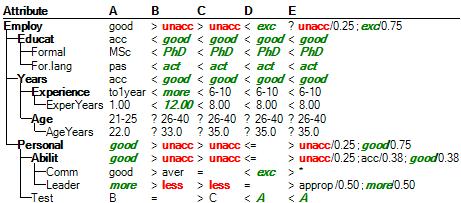
In the above display, the first alternative (candidate A) is compared in a pairwise way with the remaining ones. Operators denote the correponding preferential relations:
=: indifference, the values are equal
>: strong preference: the left-hand value is better than the right-hand one
<: strong preference: the left-hand value is worse than the right-hand one
<=: weak preference: the left-hand value is worse than or equal to the right-hand one
>=: weak preference: the left-hand value is better than or equal to the right-hand one
‘?’: unknown preference relation (due to unordered value scales or incomparable values)
Qualitative-Quantitative (QQ2) Evaluation
In addition to normal qualitative evaluation of alternatives, Qualitative-Quantitative evaluation attempts to rank altenatives within qualitative evaluations. To this end, a numeric offset is assigned to each qualitative evaluation. The maximum range of offsets is [-0.5, +0.5]: the higher the numeric offset, the better the evaluation relative to other evaluations of the same attribute. For instance, ‘good-0.27’ denotes a somewhat “bad” ‘good’ value, while ‘good+0.17’ is much better. Zero offsets are not displayed; ‘good’ actually means ‘good+0.0’.
Charts
This example shows some charts that can be obtained in DEXiWin. The charts differ in the number of evaluation dimensions and chart settings.
Bar Chart
This chart displays evaluation results according to one evaluation dimension. In this case, this is the root attribute Employ, so the chart shows the overall evaluation of the five candidates.
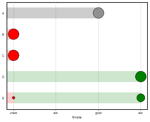
The evaluation of candidate E is distributed between ‘unacc’ and ‘exc’. Point diameters indicate the relative difference of the corresponding probabilities, 0.25 and 0.75.
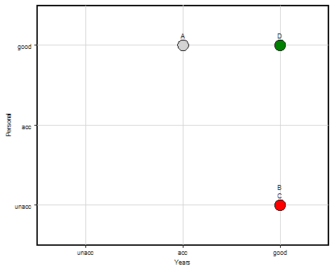
Scatter Chart
A scatter chart displays evaluation results according to two selected evaluation dimensions. In this case, the selected dimensions are Personal and Years. The candidate E is excluded from this chart.
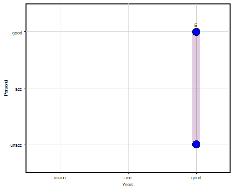
The following is the scatter chart of E, illustrating the display of value distributions:
Charts Displaying Three or More Attributes
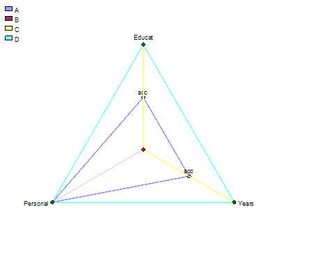
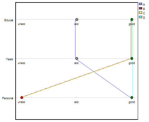
There are three types of charts that display evaluation results using three or more selected attributes: linear, radar and radar grid. Examples below show all of them. The second-level attributes Educat, Years and Personal have been selected as main chart dimensions. Candidate E has been excluded for clarity.
Linear Chart
Radar Grid Chart
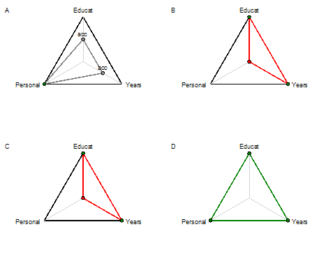
Radar Chart