Evaluation of Alternatives
With DEX models, alternatives are evaluated in the following way:
Each alternative is represented by a vector of basic attribute values.
The values of each alternatives are aggregated in a bottom-up way according to the defined structure of the model and corresponding functions.
The overall evaluation of an alternative is finally obtained as the value of one or more root attributes of the model.
On this basis, the decision maker can compare and rank the alternatives, and possibly identify and select the best one.
A more detailed description of the process depends on the type of DEX values used: single values, intervals, sets, or value distributions. Actually, the latter is the most general and covers all cases, but is also the most complex. So let us begin with simple cases. For illustration, we use the PRICE aggregation function from the Car Evaluation model.
Before that, it should be noted that DEX values include the value undefined. In principle, evaluation involving an undefined value yields an undefined results. In DEX, as an exception, is is possible to declare that any undefined value is interpreted as a full set of values of the corresponding qualitative attribute. In this case, the set-based evaluation takes place.
Single-Value Evaluation
The simplest case occurs when all input values of an alternative are defined and represented by single values. In this case, only a simple table lookup is required to find the resulting value.
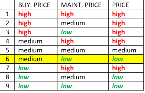
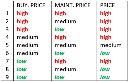
This table shows the evaluation with two single-value inputs: BUY. PRICE = ‘medium’ and MAINT. PRICE = ‘low’. The table lookup finds the corresponding decision rule 6, which yields the evaluation PRICE = ‘low’. This single value is used for further evaluation in the tree above PRICE.
Interval and Set-Based Evaluation
In this case, input values consist of intervals or sets. Several lookups in the table are generally required, one for each possible combination of input values.
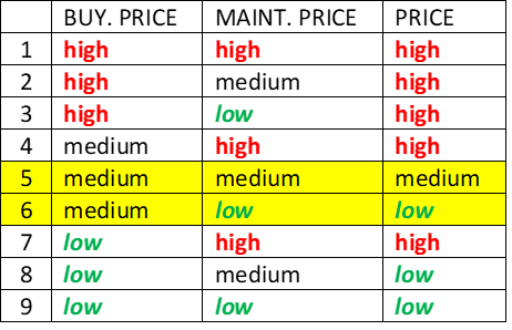
This table shows the chase when MAINT. PRICE is represented as an interval consisting of two values, ‘medium’ and ‘low’. Two rules correspond to this situation, 5 and 6. Rule 5 yields ‘medium’ and rule 6 yields ‘low’, giving the resulting interval/set PRICE = ‘medium:low’.
Distribution-Based Evaluation
The most general qualitative evaluation type occurs when input values are represented with value distributions. The evaluation considers all possible combinations of discrete input values together with probability/membership numbers p assigned to each input value.
Using Probability Distributions
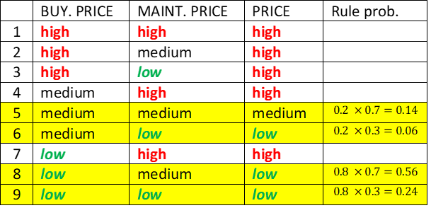
Consider input values represented with probability distributions: BUY. PRICE = ‘medium/0.2; low/0.8’ and MAINT. PRICE = ‘medium/0.7, low/0.3’. There are four possible combinations of input values, highlighted in the table. For each combination, its probability is determined as a product of the corresponding p values. Three combinations (rules 6, 8, and 9) yield value ‘low’, and one combination (rule 5) yields ‘medium’. Summing up the corresponding yield probabilities gives the final evaluation: PRICE = ‘medium/0.14; low/0.86’.
Using Fuzzy Distributions
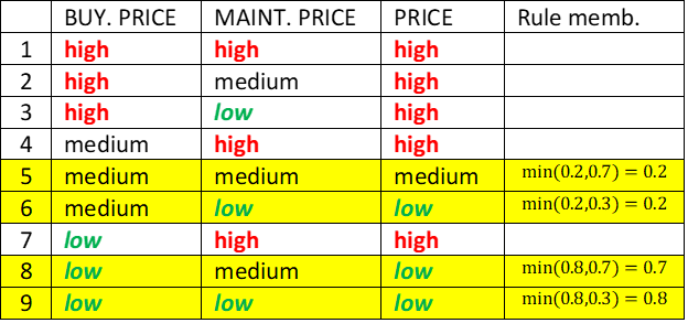
In fuzzy evaluation, input values are interpreted as fuzzy distributions and the corresponding p values as set memberships. The evaluation proceeds similarly as with probability distributions, except that product and summation operators are replaced with the minimum and maximum, respectively. Cumulative result, determined as a maximum of corresponding value yields, is PRICE = ‘medium/0.2; low/0.8’.
Qualitative-Quantitative (QQ) Evaluation
All evaluation methods described above are qualitative and assign decision alternatives to some, usually small, number of qualitative evaluations. In principle, alternatives assigned to the same “bucket” are indistinguishable between each other and cannot be ranked further. This is often undesirable in practice, particularly when the number of alternatives is large and many are in qualitative terms evaluated the same.
Looking at the above decision table, one can notice that there are as many as five rules yielding the value PRICE = high (rules 1, 2, 3, 4, 7). Comparing these rules, we can see that some rules correspond to better situations that other rules, despite the same outcome. For instance, an alternative corresponding to rule 3 (where MAINT.PRICE = low) is better or at least as good as those corresponding to rule 2 (MAINT.PRICE = medium) or rule 1 (MAINT.PRICE = high). When comparing those alternatives, the former alternative may be considered better than the latter two and thus ranked higher.
Qualitative-Quantitative (QQ) evaluation method supports such ranking by comparing decision rules in a given decision table and assigning offsets to them. Offsets are numbers on the interval [-0.5, +0.5] and reflect the internal ordering of rules (considering dominance) within each output value. The larger the offset, the better the input value combination represented by the rule.
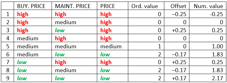
The above table illustrates the principle. The column Ord.value shows ordinal values 0, 1, 2 of the corresponding values of PRICE: high, medium and low. Offsets, calculated by the method QQ2, are shown in the column Offset. The rules 1, 2 and 3, discussed above, are indeed ranked so that 1 is the worst (-0.25) and 3 is the best (+0.25) of them. Rule 4 has the same offset as rule 2 (0), and rule 7 the same as rule 3 (+0.25). Also, rule 9 (with offset +0.17) is better than rule 8 (-0.17).
The column Num.value shows the sums of ordinal values and corresponding offsets, giving numerical values that are actually used to rank alternatives.