Examples
A typical DEXiPy workflow
This example uses a simple DEXi model for evaluating cars, which is distributed together with the DEXi software (including DEXiPy) and is used throughout DEX literature to illustrate the methodological approach (https://en.wikipedia.org/wiki/Decision_EXpert).
First, this model is loaded and printed as follows:
>>> import dexipy.dexi as dxi
>>> car = dxi.read_dexi("data/car.dxi")
>>> print(car)
DEXi Model: CAR_MODEL
Description: Car demo
index id          structure        scale                     funct
    0 CAR_MODEL   CAR_MODEL
    1 CAR         +- CAR           unacc; acc; good; exc (+) 12 3x4
    2 PRICE       |- PRICE         high; medium; low (+)     9 3x3
    3 BUY.PRICE   | |- BUY.PRICE   high; medium; low (+)
    4 MAINT.PRICE | +- MAINT.PRICE high; medium; low (+)
    5 TECH.CHAR.  +- TECH.CHAR.    bad; acc; good; exc (+)   9 3x3
    6 COMFORT     |- COMFORT       small; medium; high (+)   36 3x4x3
    7 #PERS       | |- #PERS       to_2; 3-4; more (+)
    8 #DOORS      | |- #DOORS      2; 3; 4; more (+)
    9 LUGGAGE     | +- LUGGAGE     small; medium; big (+)
   10 SAFETY      +- SAFETY        small; medium; high (+)
Rows in the printout correspond to individual attributes. The columns display:
index: Indices of attributes.
id: Unique attribute IDs, generated by DEXiPy from original DEXi names, in order to assure unambiguous referencing of attributes.
structure: The hierarchical structure of attributes, named as in the original DEXi model.
scale: Value scales associated with each attribute. The symbol
(+)indicates that the corresponding scale is ordered preferentially in an increasing order.funct: Information about the size (number of rules) and dimensions of the corresponding decision tables.
Looking at the structure of attributes, please notice that the attribute at index 0 is virtual and does not appear in the original DEXi model. In DEXiPy it allows using models that have multiple root attributes; these models appear as subtrees of the virtual root.
The “real” root of CAR_MODEL is actually CAR at index 1. It depends on two lower-level attributes, PRICE and TECH.CHAR. These are decomposed further. Overall, the model consists of:
six input (basic) attributes: BUY.PRICE, MAINT.PRICE, #PERS, #DOORS, LUGGAGE and SAFETY, and
four output (aggregate) attributes: CAR, PRICE, TECH.CHAR. and COMFORT.
Among the latter, CAR is the most important and represents the overall evaluation of cars.
The next step usually consists of defining a decision alternative or a list of alternatives
(i.e., cars in this case). The Car model already comes with a list of two cars, accessible
using dexipy.dexi.DexiModel.alternatives.
Each alternative is represented as a dictionary:
>>> car.alternatives[0]
{'name': 'Car1', 'CAR': 3, 'PRICE': 2, 'BUY.PRICE': 1, 'MAINT.PRICE': 2,
'TECH.CHAR.': 3, 'COMFORT': 2, '#PERS': 2, '#DOORS': 2, 'LUGGAGE': 2,
'SAFETY': 2}
Alternatives can be printed in a tabular form:
>>> print(car.alt_table())
alternative Car1 Car2
CAR            3    2
PRICE          2    1
BUY.PRICE      1    1
MAINT.PRICE    2    1
TECH.CHAR.     3    2
COMFORT        2    2
#PERS          2    2
#DOORS         2    2
LUGGAGE        2    2
SAFETY         2    1
In this printout, attribute values are shown using the internal DEXiPy representation,
i.e., using ordinal value numbers.
A more readable output can be obtained by dexipy.dexi.DexiModel.alt_text():
>>> print(car.alt_text())
alternative   Car1   Car2
CAR            exc   good
PRICE          low medium
BUY.PRICE   medium medium
MAINT.PRICE    low medium
TECH.CHAR.     exc   good
COMFORT       high   high
#PERS         more   more
#DOORS           4      4
LUGGAGE        big    big
SAFETY        high medium
This data can be edited using common Python list and dictionary functions.
Additionally, DEXiPy provides the method dexipy.dexi.DexiModel.alternative()
for defining a single decision alternative, for example:
>>> alt = car.alternative("MyCar1", values =
          {'BUY.PRICE': "low", 'MAINT.PRICE': 2, '#PERS': "more", '#DOORS': "4",
           'LUGGAGE': 2, 'SAFETY': "medium"})
>>> print(car.alt_table(alt))
alternative MyCar1
CAR           None
PRICE         None
BUY.PRICE      low
MAINT.PRICE      2
TECH.CHAR.    None
COMFORT       None
#PERS         more
#DOORS           4
LUGGAGE          2
SAFETY      medium
Finally, alternatives can be evaluated using dexipy.dexi.DexiModel.evaluate():
>>> eval_alt = car.evaluate(alt)
>>> print(car.alt_text(eval_alt))
alternative MyCar1
CAR            exc
PRICE          low
BUY.PRICE      low
MAINT.PRICE    low
TECH.CHAR.    good
COMFORT       high
#PERS         more
#DOORS           4
LUGGAGE        big
SAFETY      medium
Examples of using value sets and distributions
For example, let us consider a car for which we have no evidence about its possible maintenance costs.
For the value of MAINT.PRICE, we may use "*" to denote the full range of
the corresponding attribute values
(in this case equivalent to {0, 1, 2} or ('high', 'medium', 'low').
Notice how the evaluation method considers all the possible values of MAINT.PRICE
and propagates them upwards the model structure.
>>> alt = car.alternative("MyCar1a", values =
          {'BUY.PRICE': "low", 'MAINT.PRICE': "*", '#PERS': "more", '#DOORS': "4",
           'LUGGAGE': 2, 'SAFETY': "medium"})
>>> eval_alt = car.evaluate(alt)
>>> print(car.alt_text(eval_alt))
alternative                   MyCar1a
CAR                  ('unacc', 'exc')
PRICE                 ('high', 'low')
BUY.PRICE                         low
MAINT.PRICE ('high', 'medium', 'low')
TECH.CHAR.                       good
COMFORT                          high
#PERS                            more
#DOORS                              4
LUGGAGE                           big
SAFETY                         medium
The above result is not really useful, as the car turns out to be ('unacc', 'exc'), that is,
either "unacc" or "exc", depending on maintenance costs. Thus, let us try using value distribution for
MAINT.PRICE, telling DEXiPy that high maintenance costs are somewhat unexpected
(with probability p = 0.1) and that medium costs (p = 0.6) are more likely than low (p = 0.3).
The evaluation method "prob" gives the following results:
>>> alt = car.alternative("MyCar1b", values =
          {'BUY.PRICE': "low", 'MAINT.PRICE': {"low": 0.3, "medium": 0.6, "high": 0.1},
           '#PERS': "more", '#DOORS': "4", 'LUGGAGE': 2, 'SAFETY': "medium"})
>>> eval_alt = car.evaluate(alt, method = "prob")
>>> print(car.alt_text(eval_alt, decimals = 2))
alternative                                  MyCar1b
CAR                       {'unacc': 0.1, 'exc': 0.9}
PRICE                      {'high': 0.1, 'low': 0.9}
BUY.PRICE                                        low
MAINT.PRICE {'high': 0.1, 'medium': 0.6, 'low': 0.3}
TECH.CHAR.                                      good
COMFORT                                         high
#PERS                                           more
#DOORS                                             4
LUGGAGE                                          big
SAFETY                                        medium
In this case, the final evaluation of CAR is {'unacc': 0.1, 'exc': 0.9}, that is,
it is much more likely that MyCar1b is "exc" than "unacc".
Analysis of alternatives
In DEXiPy, the evaluation of alternatives can be enhanced by analysis. There are three main analysis methods implemented in DEXiPy: selective explanation, plus/minus analysis and `comparison of alternatives. The following examples illustrate these analyses using the two alternatives, Car1 and Car2, included in the Car.dxi model.
Selective explanation prints out particularly bad and particularly good evaluations:
>>> car.selective_explanation()
Alternative Car1
Weak points
None
Strong points
attribute         Car1
+-CAR              exc
  |-PRICE          low
  | +-MAINT.PRICE  low
  +-TECH.CHAR.     exc
    |-COMFORT     high
    | |-#PERS     more
    | +-LUGGAGE    big
    +-SAFETY      high
Alternative Car2
Weak points
None
Strong points
attribute       Car2
    |-COMFORT   high
    | |-#PERS   more
    | +-LUGGAGE  big
Plus/minus analysis investigates the effects of changing one attribute value at a time. For example, considering alternative Car2:
>>> car.plus_minus(car.alternatives[1])
Attribute         -2    -1    Car2   +1  +2
CAR                           good
  | |-BUY.PRICE   [     unacc medium exc ]
  | +-MAINT.PRICE [     unacc medium exc ]
    | |-#PERS     unacc       more   ]
    | |-#DOORS    unacc       4          ]
    | +-LUGGAGE   unacc       big    ]
    +-SAFETY      [     unacc medium exc ]
Here, the column Car2 shows the current situation, where the overall value of Car2 is “good”.
The columns labelled from -2 to +2 display overall evaluations
(i.e., values of the CAR attribute) in the cases when the values of
corresponding attributes change for the indicated number of qualitative steps.
For instance, if BUY.PRICE takes a one step lower value
(-1, from “medium” to “high”; the latter is not shown explicitly),
the overall CAR evaluation would have become “unacc”.
Similarly, if SAFETY improves by +1, i.e., from “medium” to “high”,
the overall evaluation improves to “exc”.
The backets [ and ] indicate positions that exceed scale limits.
Compare alternatives compares an alternative with other alternatives. For instance, comparison of Car1 with Car2:
>>> car.compare_alternatives(car.alternatives[0], car.alternatives[1])
Attribute         Car1   Car2
+-CAR             exc    > good
  |-PRICE         low    > medium
  | |-BUY.PRICE   medium =
  | +-MAINT.PRICE low    > medium
  +-TECH.CHAR.    exc    > good
    |-COMFORT     high   =
    | |-#PERS     more   =
    | |-#DOORS    4      =
    | +-LUGGAGE   big    =
    +-SAFETY      high   > medium
Charts
DEXiPy provides several methods for drawing alternatives’ data and evaluation results:
plotalt1: Plots multiple alternatives with respect to a single attribute:
>>> plotalt1(car)

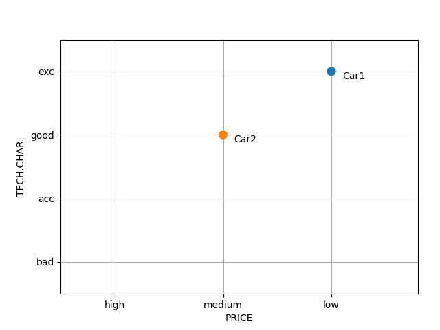
plotalt2: A scatterplot of multiple alternatives with respect to two attributes:
>>> plotalt2(car, "PRICE", "TECH.CHAR.")
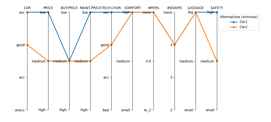
plotalt_parallel: Plots multiple alternatives with respect to multiple attributes, using parallel axes:
>>> plotalt_parallel(car)
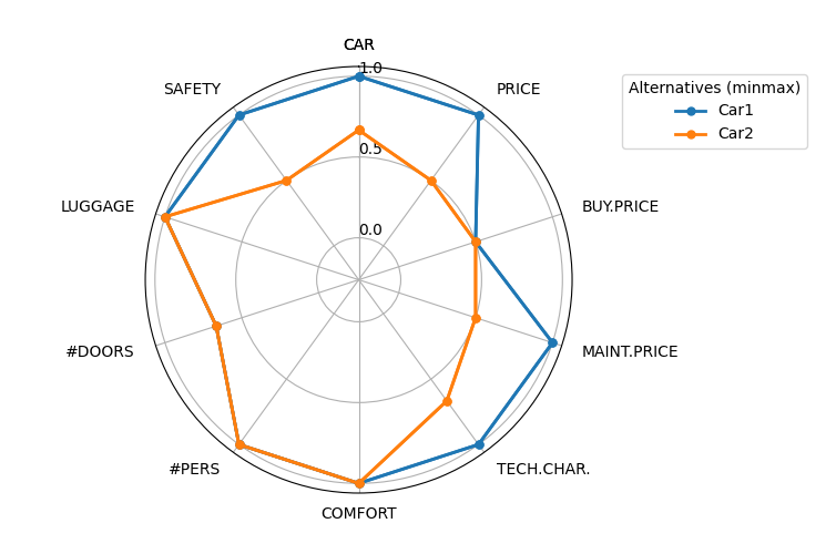
plotalt_radar: Plots multiple alternatives with respect to multiple attributes, using a “radar” chart:
>>> plotalt_radar(car)
Writing alternatives
Any alternatives, either read to or created in DEXiPy Python environment, can be written to an external tab-delimited or csv-type file, which can be subsequently imported to the DEXi or DEXiWin software.
When the filename argument is “”, as in the following examples, file contents is written to the console:
>>> import csv
>>> # use csv format
>>> write_alternatives(car, car.alternatives, "", quotechar = '"', quoting = csv.QUOTE_ALL)
"name","Car1","Car2"
"CAR","4","3"
". PRICE","3","2"
". . BUY.PRICE","2","2"
". . MAINT.PRICE","3","2"
". TECH.CHAR.","4","3"
". . COMFORT","3","3"
". . . #PERS","3","3"
". . . #DOORS","3","3"
". . . LUGGAGE","3","3"
". . SAFETY","3","2"
>>> # use tab-delimited format
>>> write_alternatives(car, car.alternatives, "", delimiter = "\t")
name    Car1    Car2
CAR     4       3
. PRICE 3       2
. . BUY.PRICE   2       2
. . MAINT.PRICE 3       2
. TECH.CHAR.    4       3
. . COMFORT     3       3
. . . #PERS     3       3
. . . #DOORS    3       3
. . . LUGGAGE   3       3
. . SAFETY      3       2